TL;DR

Finally to the agenda: Neural networks. In this post we’ll cover categorization problem using softmax classifier. All the code in this post is written in Python, version 3.6. I’ve gathered most of the used material from here.

Neural networks

Sorry, but this is going to be quite a long post, since there’s a lot of stuff we have to go through. In the previous posts we’ve been doing “linear analysis”, or we could say that the functions which we’ve fitted were linear. Neural networks enables us to fit our functions to non-linear data, which can be a huge advantage in some cases (f.ex. speech & image recognition). As before, let’s create some data first, so that we can visualize the problem.

%matplotlib inline
import numpy as np
import matplotlib.pyplot as plt
import matplotlib
from IPython.display import Image
from IPython.core.display import HTML

matplotlib.rcParams['figure.figsize'] = (15.0, 10.0)


num_of_points = 1500

# This is our magic function for classifying points
def magic_function(x, y):
    y_val = np.sin(np.pi*x / 2.) - np.random.rand() * 1.2
    if y_val < y:
        return 0
    if x > -1 - np.random.rand() / 2.:
        return 1
    else:
        return 2

# Let's generate some points
x = np.random.normal(-1, 2, num_of_points)
y = np.random.normal(-1, 1, num_of_points)
n = np.array([magic_function(i, j) for i, j in zip(x, y)])

# Combine data
train_input = np.array([x,y]).T
train_output = np.array(n)

# Shuffle the points
perm = np.random.permutation(train_output.shape[0])
train_input_shuffled = train_input[perm]
train_output_shuffled = train_output[perm]

# plot plot
plt.scatter( x, y, c=n)
plt.grid()

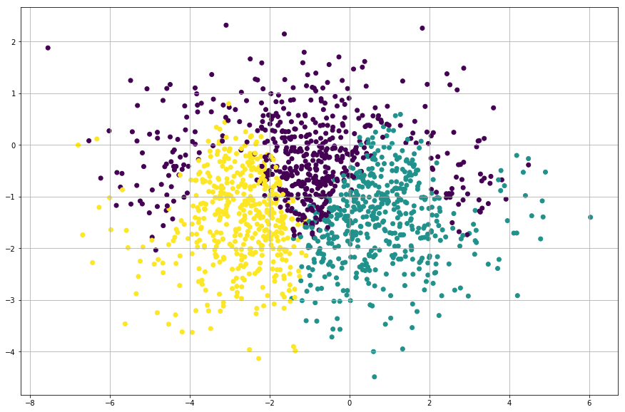
It’s quite hard to fit a linear function to this data. We’ll start our journey to neural network from the basics and we’ll begin with “feed forward”…

Feed forward

As I’ve studied more on neural networks, majority of the websites tended to start with brain analogy: neurons inside the brain and how neurons are connected with each other. For me this approach proved to be super confusing, so I’m just gonna skip that and go with the mathematical analogies (and later I try to draw some circles…). Nevertheless, our goal remains the same: we’re just trying to fit our function to some given data by finding the optimal multipliers.

Let’s first start with the feed forward or forward pass. As the name suggests, we have something, and feed it forward. In our case we have a function, which produces a results $y$, which we again feed to another function. Instead of one, we have some $x$ number of functions. In the Logistic regression post we used sigmoid function, but this function is only capable of presenting binary values: $1$ or $0$. This is quite undesirable, when there are more than two categories. There are couple of choices which we could use, but we’ll go with the rectified linear unit function or in short, ReLU:

\begin{equation} f_{ReLU} = max(0, x) \end{equation}

We’re still going to use linear functions, which we will feed into the ReLU function:

\begin{equation} f(x, \theta, b) = \theta^T x + b \end{equation}

In this post I’m going to use following notation:

\begin{equation} (x, \theta, b) \rightarrow f(x, \theta, b) \rightarrow \mathcal{O} \end{equation}

in which $\mathcal{O}$ is the output of the function. We should start with an example, how to implement this. Let’s create two (2) functions and create a pipe, where one feeds it’s result to another function:

linear_function = lambda a, b, x: np.dot(a, x) + b

def relu(x):
    """Sigmoid function https://en.wikipedia.org/wiki/Sigmoid_function
    """
    return np.maximum(0, x)

# functions 1 and 2
f1 = lambda x: relu(linear_function(1.8, 2.4, x))
f2 = lambda x: relu(linear_function(2.4, -2.2, x))

# Our pipe
f3 = lambda x: f2(f1(x))

# x values
x = np.linspace(-10, 10, 200)

# Results for each function
f1_results = f1(x)
f2_results = f2(x)

# Results for feed forward
feed_forward_results = f3(x)

# plotting
matplotlib.rcParams['figure.figsize'] = (15.0, 10.0)
plt.plot(x, feed_forward_results, 'r--', label="$f3=f_2(f_1(x))$")
plt.plot(x, f1_results, 'k', label="$f1$")
plt.plot(x, f2_results, 'b', label="$f2$")
plt.legend()
plt.grid()

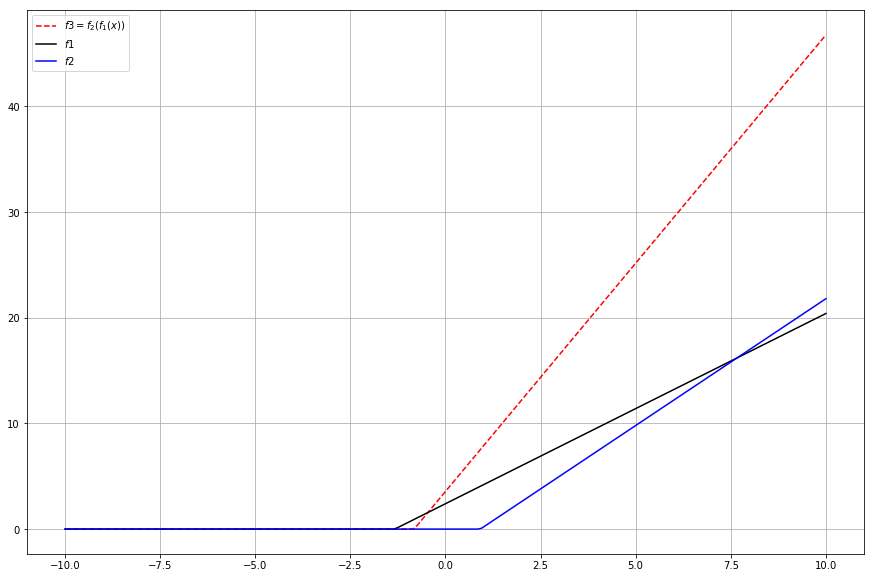
Well, that doesn’t seem to be that useful at all. But wait! Fun part is yet to come. If you look at the code, you can notice how I put both $f_1$ and $f_2$ their own multipliers. We can like to visualize with some arrows:

\begin{equation} x \rightarrow f_1(x) \rightarrow f_2(\mathcal{O_1}) \rightarrow y \end{equation}

Now to the terminology: Our pipe represent our neural network and each functions present a layer. $f_1$ is input layer and $f_2$ is the output layer. If we would have more functions between $f_1$ and $f_2$, they would be called just a hidden layers. There can be N-number of hidden layers, but just for naming conventions, first is input layer and last output. And don’t think it too hard… I tried and got confused.

Ok, easy peasy. Now to the fun part. What about if we increase the number of multipliers in each layer? This should pose no problem, since we’re using dot function, which will take care of sum and product operations (We just have to make sure all the matrices have proper shapes, because feed forward). We will be using a matrix for storing the multipliers, so we can choose the length (read height) and width. Let’s try with a case, where:

• $f_1$ multiplier matrix has length 5 and width 1
• $f_2$ multiplier matrix has length 1 and width 5

And if we expand the pipe:

\begin{equation} x \rightarrow f_1(x) \rightarrow f_2(\mathcal{O_1}) \rightarrow y \end{equation}

Let’s give it a try:

# I'll be using normal distribution for scattering the multiplier values
# I've picked mean and deviation values on random

# First function definitions
f1_matrix_length = 5
f1_matrix_width = 1
theta_a = np.random.normal(0.15, 1.4, (f1_matrix_length, f1_matrix_width))
b_a = np.random.normal(-1.2, 2.3, f1_matrix_length)

# Second function definitions
f2_matrix_length = 1
f2_matrix_width = 5
theta_b = np.random.normal(0.5, 2.2, (f2_matrix_length, f2_matrix_width))
b_b = np.random.normal(-0.12, 2, f2_matrix_length)

# Function wrappers
f1 = lambda x: relu(linear_function(theta_a, b_a, x))
f2 = lambda x: relu(linear_function(theta_b, b_b, x))

# Our pipe
feed_forward = lambda x: f2(f1(x))

# Calculate a result for given x
x = np.linspace(-10, 10, 200)
feed_forward_results = np.zeros(200)
for idx, xi in enumerate(x):
    feed_forward_results[idx] = feed_forward([xi])

# Plotting
matplotlib.rcParams['figure.figsize'] = (15.0, 10.0)
plt.plot(x, feed_forward_results, 'r--', label="$feedforward=f_2(f_1(x))$")
plt.legend()
plt.grid()

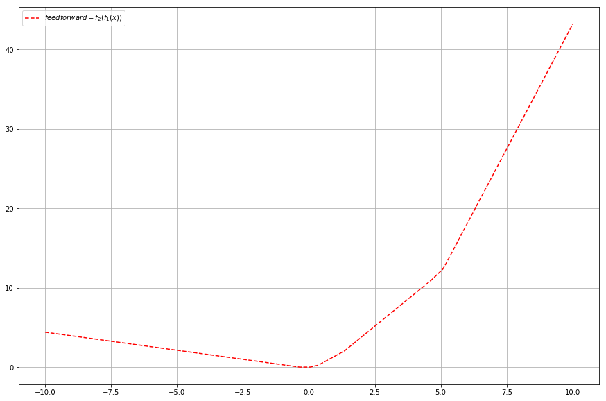
That’s more like it. I’d say quite interesting shape. We only applied one extra dimension to our matrices, but what if we add a second one? And since we’re going crazy why not throw an extra function $f_3$. Let’s decide that the first matrix now has shape (5,2) so the input $x$ has to have shape (2).

\begin{equation} x \rightarrow f_1(x) \rightarrow f_2(\mathcal{O_1}) \rightarrow f_3(\mathcal{O_2}) \rightarrow y \end{equation}

# Once again, I'll be using normal distribution for scattering the multiplier values

# First function definitions
f1_num_of_neurons = 5
f1_num_of_multipliers = 2
theta_a = np.random.normal(0.5, 1.4, (f1_num_of_neurons, f1_num_of_multipliers))
b_a = np.random.normal(-1.2, 2.3, f1_num_of_neurons)

# Second function definitions
f2_num_of_neurons = 2
f2_num_of_multipliers = f1_num_of_neurons
theta_b = np.random.normal(1.5, 3.2, (f2_num_of_neurons, f2_num_of_multipliers))
b_b = np.random.normal(-0.12, 2, f2_num_of_neurons)

# Third function definitions
f3_num_of_neurons = 1
f3_num_of_multipliers = f2_num_of_neurons
theta_c = np.random.normal(2.4, 0.19, (f3_num_of_neurons, f3_num_of_multipliers))
b_c = np.random.normal(-2, 2, f3_num_of_neurons)

# Function wrappers
f1 = lambda x: relu(linear_function(theta_a, b_a, x))
f2 = lambda x: relu(linear_function(theta_b, b_b, x))
f3 = lambda x: relu(linear_function(theta_c, b_c, x))

# Pipe
feed_forward = lambda x: f3(f2(f1(x)))

# Calculate points for grid
num_points = 100
x_1 = np.linspace(-10, 10, num_points)
x_2 = np.linspace(-10, 10, num_points)

feed_forward_results = np.zeros((num_points, num_points))
for x_, x_i in enumerate(x_1):
    for y_, x_j in enumerate(x_2):
        value = feed_forward([x_i, x_j])[0]
        feed_forward_results[x_, y_] = value

# Plotting
X, Y = np.meshgrid(x_1, x_2)
matplotlib.rcParams['figure.figsize'] = (15.0, 10.0)
cs = plt.contourf(X, Y, feed_forward_results)
plt.colorbar(cs)
plt.grid()

Whoa, such matrix joggling… let’s stop for a second and review some analogies. Less math is sometimes good for everybody :)

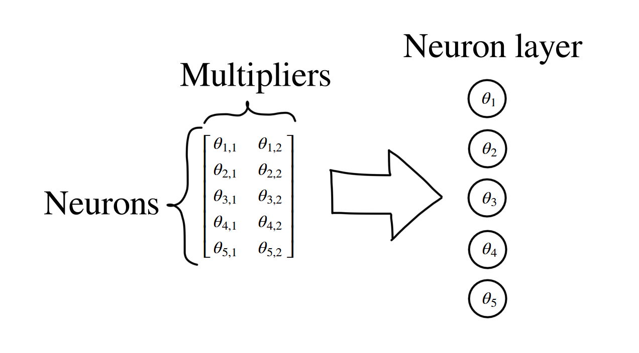
As we talked before, each function represents a layer. In each function, each row in multiplier matrix represents a neuron. Usually (at least the pages where I visited) the multiplier columns aren’t drawn. This leaves us with the circles, which represent only the neurons. In the picture above we can see that our matrix represents five (5) neurons. With the given analogy, we can draw our last example network as:

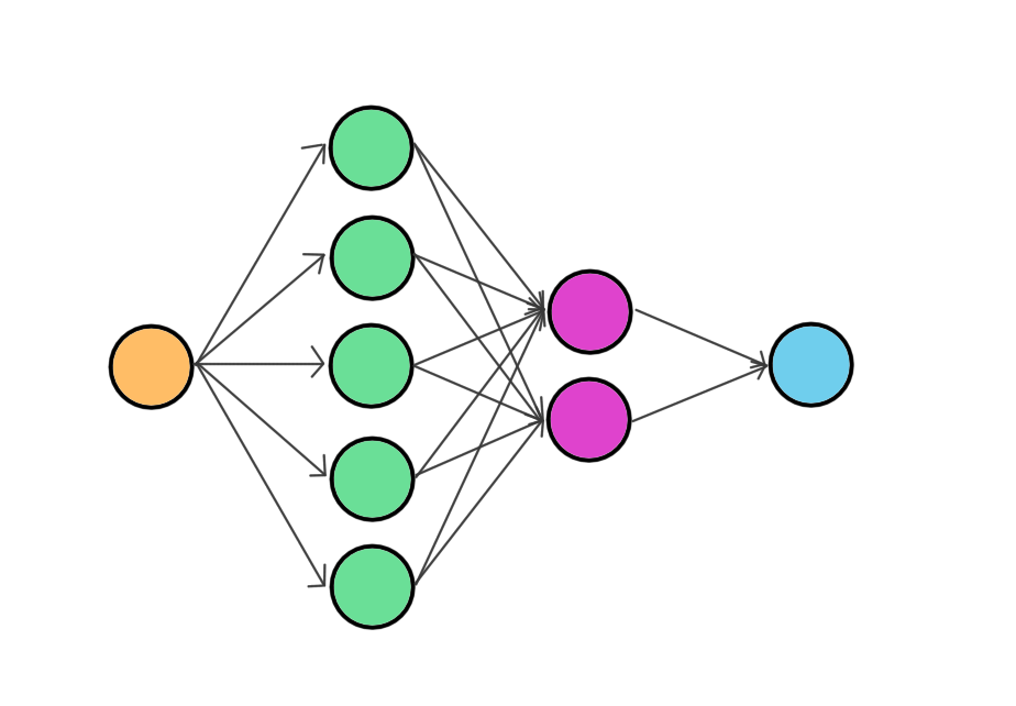
and thus the name: neural network. Arrows just show how values are applied to the neuron (dot product and sum). If you’re still reading: Congratulations! I have to honest: we’ve only covered the first half here, but do not worry! Following stuff is almost the same as in the previous posts. No dragons or nightmares.

Softmax classifier

Classification using propabilities

In the last post we used support vector machine (SVM) for categorization problem but now we’re about to use softmax classifier. Softmax is defined as:

\begin{equation} L_i = -\log(p_{y_i}), \hspace{1cm} p_k = \frac{e^{f_k}}{\sum_j e^{f_{j}}} \end{equation}

and if we use logaritmic rules, we can derive:

\begin{equation} L_i = -\log\bigg( \frac{e^{f_{y_i}}}{\sum_j e^{f_{j}}} \bigg) \end{equation}

\begin{equation} L_i = -\bigg( \log\big(e^{f_{y_i}}\big) - log \big(\sum_j e^{f_{j}} \big) \bigg) \end{equation}

\begin{equation} L_i = log \big(\sum_j e^{f_{j}} \big) -f_{y_i} \end{equation}

SVM produced a score for each class, but softmax produces a probability. Just to see how this function works, let’s calculate the same example as in the last post: input vector has six (6) elements and in the output we should have four (4) classes.

input_vector = np.array([5.2, 1.0, 6.356, 10.1, -4.45, 8.20]).T
theta = np.random.rand(4,6)
yi = np.array([1])
scores = np.dot(theta, input_vector)
exp_scores = np.exp(scores)
probs = exp_scores / np.sum(exp_scores)
print("Propabilities: {0}".format(probs))
Li = -np.log(probs[yi])[0]
print("Score: {0}".format(Li))

Probabilities: [  8.50640639e-05   7.16811307e-03   3.23025170e-06   9.92743593e-01]
Score: 4.938112829809168

In our total loss function we apply again a regularization loss (the same $L_2$ as in the last post and since our network has multiple multipliers, let’s sum these together), which leaves us with:

\begin{equation} L = \frac{1}{N}\sum_i L_i + \frac{\lambda}{2} \sum_j R(\theta_j) \end{equation}

in which $j$ is the number of $\theta$’s or layers. We still need calculate the gradient for the stochastic gradient descent. Luckily we can use calculus for this task.

\begin{equation} \frac{\partial L}{\partial f_k} = \frac{\partial }{\partial f_k} \Bigg( log \big(\sum_j e^{f_{j}} \big) -f_{y_i} \Bigg) \end{equation}

Let’s use derivate rules of logarithm to derivate our function: $\frac{d}{dx} \log(x^n) = \frac{nx^{n-1}}{x^n}$

\begin{equation} \frac{\partial L}{\partial f_k} = \frac{e^{f_{k}}}{\sum_j e^{f_{j}}} - \mathbb{1}(y_i = k) \end{equation}

\begin{equation} \frac{\partial L}{\partial f_k} = p_k - \mathbb{1}(y_i = k) \end{equation}

Easy peasy. I used the code from this site, since I didn’t want to add my mistakes here.

def softmax_classifier(scores, y):
    """
    Softmax classifier, reference: http://cs231n.github.io/neural-networks-case-study/

    Parameters
    ----------
        scores: array, size: NxM
            Score array for each data point
        y: array, size: N
            Correct indeces for each data point
    """
    n_values = len(y)
    exp_scores = np.exp(scores)
    probs = exp_scores / np.sum(exp_scores, axis=1, keepdims=True)

    # compute the loss: average cross-entropy loss and regularization
    correct_logprobs = -np.log(probs[range(n_values),y])
    data_loss = np.sum(correct_logprobs) / n_values

    dscores = probs
    dscores[range(n_values),y] -= 1
    dscores /= n_values
    return data_loss, dscores

Back propagation

In the last post we only had one function for fitting. Updating the multipliers in the optimization loop was quite easy but think a bit our new situation: we have an input, we feed it into a network and get an output. We have no idea, what kind of effect each layer had on the result. Solution to this problem is back propagation. In principle is we count backwards how much a given layer had an effect.

This requires some serious chain rule derivation and here’s a couple of derivatives for our upcoming neural network with three layers:

\begin{equation} \frac{\partial L}{\partial \theta_3} = \frac{\partial L}{\partial \mathcal{O_3}} \frac{\partial \mathcal{O_3}}{\partial \theta_3} + \lambda \theta_3 \rightarrow \frac{\partial L}{\partial f_k} \mathcal{O_2} + \lambda \theta_3 \end{equation}

\begin{equation} \frac{\partial L}{\partial b_3} = \frac{\partial L}{\partial \mathcal{O_3}} \frac{\partial \mathcal{O_3}}{\partial b_3} \rightarrow \frac{\partial L}{\partial f_k}\mathbb{1} \end{equation}

\begin{equation} \frac{\partial L}{\partial \mathcal{O_2}} = \frac{\partial L}{\partial \mathcal{O_3}} \frac{\partial \mathcal{O_3}}{\partial \mathcal{O_2}} \rightarrow \frac{\partial L}{\partial f_k}\theta_3 \end{equation}

in which $\mathbb{1}$ is array of ones. The hidden layers are derivated the same, but with more derivatives:

\begin{equation} \frac{\partial L}{\partial \theta_2} = \frac{\partial L}{\partial \mathcal{O_3}} \frac{\partial \mathcal{O_3}}{\partial \mathcal{O_2}} \frac{\partial \mathcal{O_2}}{\partial \theta_2} + \lambda \theta_2 \rightarrow \frac{\partial L}{\partial \mathcal{O_2}} \mathcal{O_1} + \lambda \theta_2 \end{equation}

\begin{equation} \frac{\partial L}{\partial b_2} = \frac{\partial L}{\partial \mathcal{O_3}} \frac{\partial \mathcal{O_3}}{\partial \mathcal{O_2}} \frac{\partial \mathcal{O_2}}{\partial b_2} \rightarrow \frac{\partial L}{\partial \mathcal{O_2}} \mathbb{1} \end{equation}

After calculating all the derivatives we can apply the gradient update, f.ex:

\begin{equation} \theta_3 = \theta_3 + \Delta \frac{\partial L}{\partial \theta_3} \end{equation}

in which $\Delta$ is the step size. Do note that f.ex. $\frac{\partial L}{\partial \theta_3}$ has to be the same shape as $\theta_3$ so this requires some matrix jugging the transposes. If you need more information, please check here and here sites for definitions and examples.

Model

Ok, let’s sum things up: we need a neural network, softmax classifier and we need to back propagate the values for the gradient update. Without further due let’s give it a try. I’ve taken some examples from here, which has been a great source for more definitions.

# Number of inputs
D = 2

# Sizes of hidden layers
hidden_size_1 = 100
hidden_size_2 = 25
output_size = 3

θ_1 = 0.01 * np.random.randn(D, hidden_size_1)
b_1 = 0.01 * np.random.randn(1, hidden_size_1)

θ_2 = 0.01 * np.random.randn(hidden_size_1, hidden_size_2)
b_2 = 0.01 * np.random.randn(1, hidden_size_2)

θ_3 = 0.01 * np.random.randn(hidden_size_2, output_size)
b_3 = 0.01 * np.random.randn(1, output_size)

X = train_input_shuffled
y = train_output_shuffled

# some hyperparameters
step_size = 0.5
λ = 1e-3 # regularization strength

b_ones = np.ones(X.shape[0])

iteration_numbers = []
losses = []

for i in range(4000):

    # Calculate scores
    O_1 = np.maximum(0, np.dot(X, θ_1) + b_1)   # note, ReLU layer
    O_2 = np.maximum(0, np.dot(O_1, θ_2) + b_2) # note, ReLU layer
    scores = np.dot(O_2, θ_3) + b_3

    # Calculate loss and gradient
    L, dL = softmax_classifier(scores, y)

    # Regularization penalty
    reg_penalty = sum([0.5 * λ * np.sum(x**2) for x in [θ_1, θ_2, θ_3]])
    total_loss = L + reg_penalty

    # Backpropagate gradients
    dθ_3 = np.dot(O_2.T, dL)
    db_3 = np.dot(b_ones, dL)

    dO_2 = np.dot(dL, θ_3.T)
    dO_2[O_2 <= 0] = 0            # Relu layer has max function, which requires this step
    dθ_2 = np.dot(O_1.T, dO_2)
    db_2 = np.dot(b_ones, dO_2)

    dO_1 = np.dot(dO_2, θ_2.T)
    dO_1[O_1 <= 0] = 0
    dθ_1 = np.dot(X.T, dO_1)
    db_1 = np.dot(b_ones, dO_1)

    # Add regularization gradient contribution
    dθ_1 += λ * θ_1
    dθ_2 += λ * θ_2
    dθ_3 += λ * θ_3

    # Perform a gradient update
    θ_1 += -step_size * dθ_1
    b_1 += -step_size * db_1

    θ_2 += -step_size * dθ_2
    b_2 += -step_size * db_2

    θ_3 += -step_size * dθ_3
    b_3 += -step_size * db_3

    # Add iteration number and loss for plotting
    iteration_numbers.append(i)
    losses.append(total_loss)

plt.plot(iteration_numbers, losses)
plt.xlabel("Iteration number")
plt.ylabel("Loss")
plt.grid()

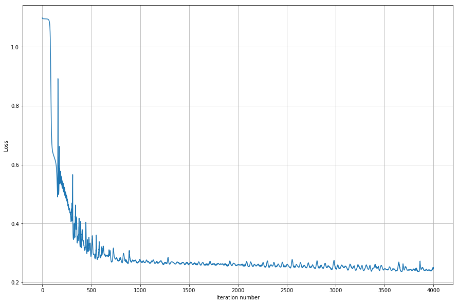
A bit spiky, but converges quite nicely so I’d say it looks promising. Let’s plot the results and see how our fit worked.

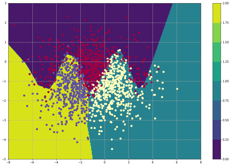
num_points = 300
x_1 = np.linspace(-8, 8, num_points)
x_2 = np.linspace(-5, 3, num_points)

feed_forward_results = np.zeros((num_points, num_points))
X1, Y2 = np.meshgrid(x_1, x_2)
for x_, row in enumerate(zip(X1, Y2)):
    for y_, vals in enumerate(zip(*row)):
        x_j, x_i = vals
        k = [x_j, x_i]
        O_1 = np.maximum(0, np.dot(k, θ_1) + b_1) # note, ReLU
        O_2 = np.maximum(0, np.dot(O_1, θ_2) + b_2) # note, ReLU
        scores = np.dot(O_2, θ_3) + b_3
        value = np.argmax(scores)
        feed_forward_results[x_, y_] = value

matplotlib.rcParams['figure.figsize'] = (15.0, 10.0)
cs = plt.contourf(X1, Y2, feed_forward_results)
plt.colorbar(cs)
plt.scatter(X[:, 0], X[:, 1], c=y, s=40, cmap=plt.cm.Spectral)
plt.grid()

Conclusion

In this post we implemented a neural network using softmax classifier. We could improve our model by checking for over fitting, improving gradient update (ref), modifing/preprocess the input data for the network (ref) and an overall code review to improve the code quality. Now the model, which we just created, is only for educational purposes, so shouldn’t use this in real analysis. I’d recommend that if you’re planning create some serious models, use f.ex. scikit-learn or tensorflow. But I guess making the best of these tools you need to know what’s happening under the hood. In the next post we’ll take a look a bit more concrete example and check how I used this to teach my bot to play halite. Hopefully you liked this post, stay tuned!