TL;DR;

In the last post we explored linear regression and familiarized some core concepts. In this post we’ll take a look in Logistic Regression. All the code is in Julia programming language. Most of the theory can be found here.

Keywords: Classification problem, binary, linear

Logistic regression

In the last post we familiarized following concepts: cost functions, computing gradients and learned how to optimize functions over a set of parameters. Linear regression is a great tool for predicting the $y$ value with given $x$ value(s). But what if I have given value(s) $x$, how can I predict whether it produces 1 or 0. This is a classification problem and logistic regression is a fine tool for this kind of problem. Let’s check Wikipedia definition:

In statistics, logistic regression, or logit regression, or logit model is a regression model where the dependent variable (DV) is categorical.

So we can solve problems, f.ex. when I know the height and weight of an animal, can I predict if it is an elephand or a rhino. Let’s create a plot so we can analyze this more.

using PyPlot
using Optim
using Distributions

# Some random x distributions
x_hornet = rand(Normal(100, 7), 600);
x_bbee = rand(Normal(110, 7), 600);

# Magic function for generating data
f_hornet(x) = 50 + 0.7 *  x .+ rand(Normal(1, 7), length(x_hornet)) .* rand(length(x_hornet))
f_bbee(x) = 35 + 0.7 *  x .+ rand(Normal(1, 7), length(x_bbee)) .* rand(length(x_bbee))

# y values for x distributions
y_hornet = f_hornet(x_hornet);
y_bbee = f_bbee(x_bbee);

#  Plot definitions
scatter(x_hornet, y_hornet, c="b", marker="+", label="Hornet")
scatter(x_bbee, y_bbee, c="r", marker="x", label="Bumblebee")
axis(:equal)
xlabel("Size of the insect")
ylabel("How terrifying insect looks")
grid()
legend()

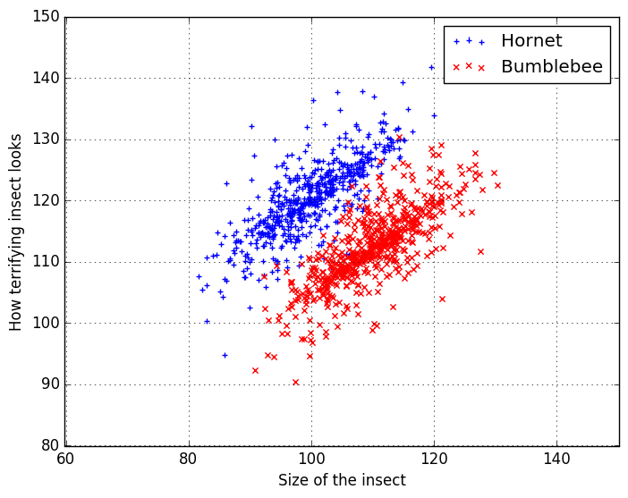
In the plot we have two distinct regions for hornets and bumblebees. If I would measure a new insect and get the values (100, 100), I could see from the plot, that it’s most probably a bumblebee. But if I would not have this plot at my disposable, it’d be quite harder to guess, which insect it would be. Luckily we can use logistic regression for this task. It operates with the same principles as linear regression, but we need to tweak a bit the cost functions and target function (which was the linear functions in the last post).

Sigmoid function

First what we need is a function, which produces binary values (1 and 0). Sigmoid function is a popular choice in AI applications, which is why we’ll also use it.

\begin{equation} f(x) = \frac{1}{1 + \exp(-x)} \end{equation}

using PyPlot

# Sigmoid function
sigmoid(x) = 1 ./ (1 + exp(-x))

# Values for plot
x_vals = collect(-10:0.1:10)
y_vals = sigmoid(x_vals)

# Plot definitions
grid()
plot(x_vals, y_vals)
xlabel(L"x", size=25)
ylabel(L"\frac{1}{(1 + \exp(-x))}", size=25)

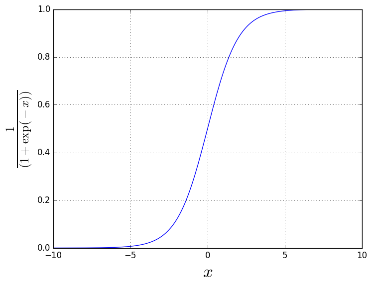
As we can see from the plot, sigmoid function produces either 1 or 0 depending on the $x$ value. But now we’re lacking the multipliers, which we were so interested in the last post. Trick now is to use the same linear functions, as in the linear regression:

\begin{equation} g(x) = \sum_i \theta_i x_i = \theta^T x \end{equation}

and shove the function inside the sigmoid function. This way we can squash the linear functions results into ones and zeros.

\begin{equation} p(x) = \frac{1}{1 + \exp(-g(x))} \rightarrow \frac{1}{1 + \exp(-\theta^T x)} \end{equation}

Now we maybe be thinking, what about the region where $x$ is almost 0. If sigmoid produces, f.ex. 0.6, how do we be interpret the result: is it a hornet or bumblebee? We need to change our way of thinking, from viewing these as a exact results, into probabilities. Question could be: is this a hornet? With probability of 1, we interpret result as true and 0 as false. If sigmoid produces 0.88, it’s quite safe to say it’s a hornet and 0.22 can be interpreted, that it’s a bumblebee. The region near 0.5 is, where we’re quite uncertain. Now that we’ve established a function, we need a way to calculate it’s fitness.

Cost function

The least squares loss function was used in the linear regression to measure the error of our fit. This is unsuitable approach now, since we measured the error to measurement points but now we’re dealing with probabilities. We need to change the cost function to measure the likelyhood of our fit. I’ve picked the definitions from here. First we need a likelyhood function:

\begin{equation} L = \prod_{i=1}^n p(x_i)^{y_i}(1-p(x_i))^{1-y_i} \end{equation}

Let’s apply log to our likelyhood function, to turn products into sums:

\begin{equation} J = \log(L) = \sum_{i=1}^n y_i \log(p(x_i)) + (1-y_i)\log(1-p(x_i)) \end{equation}

Now, that this is ready, let’s plot a small example to see how likelyhood function behaves:

using PyPlot
using Optim
using Distributions

function p_sigmoid(x)
    return 1 ./ (1. + exp(-x))
end

# Two points:
y = [0 1]
x = [0.25, 1.1]

# Multipliers
theta = collect(-2:0.05:5)
l_theta = length(theta)
J = zeros(l_theta)

# Looping all the multipliers
for i=1:l_theta
    px = p_sigmoid(x.*theta[i])
    J_ = y * log(px) + (1-y)*log(1-px)
    J[i] = J_[1]
end

# Plot definitions
grid()
plot(theta, J)
title("Cost function values")
xlabel("Multilier value")
ylabel("Likelyhood")

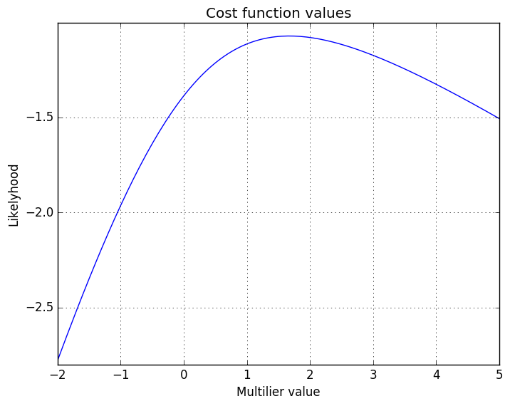
As we can see, the best likehood can be achived, when multilier is somewhere 1.5. But our curve opens downwards, not upwards. In order to use old minimization functions (gradient descent or BFGS) in our model, we need to maximize the likehood, not to minimize. Luckily, we can just flip the curve using minus sign.

J = zeros(l_theta)

# Looping all the multipliers
for i=1:l_theta
    px = p_sigmoid(x.*theta[i])
    J_ = y * log(px) + (1-y)*log(1-px)
    J[i] = -J_[1] # I'll just add minus here
end

# Plot definitions
grid()
plot(theta, J)
xlabel("Multilier value", size=20)
ylabel("Likelyhood", size=20)

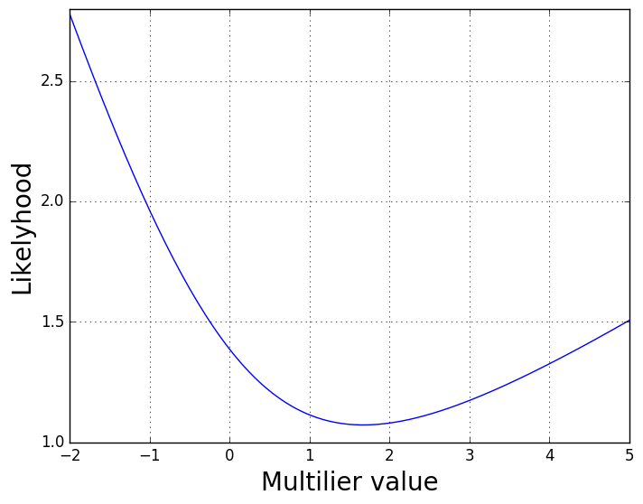
That’s much better. We’re good to go, let’s assemble our model next.

Model

Here’s a summary, what we’re using:

Tweaked sigmoid function:

\begin{equation} p(x) = \frac{1}{1 + \exp(-\theta^T x)} \end{equation}

Likelyhood cost function (gradient can also be found here):

\begin{equation} J = -\sum_{i=1}^n y_i \log(p(x_i)) + (1-y_i)\log(1-p(x_i)) , \hspace{1cm} \nabla_\theta J = \sum_{i=1}^n x_i (p(x_i) - y_i) \end{equation}

Now that we’re dealing with probabilities, gradient descent is now called stochastic gradient ascent:

\begin{equation} x_{n+1} = x_n - \gamma \nabla f(x_n) \end{equation}

Let’s start cracking!

using PyPlot
using Optim

##############################
#    Function definitions    #
##############################

""" Sigmoid function
"""
function sigmoid(O, x)
    xx = O' * x
    return 1 ./ (1. + exp(-xx))
end

"""Cost function"""
function cost(O, x, y)
    h_x = sigmoid(O, x)
    log_hx = log(h_x)'
    log_hx_neg = log(1 - h_x)'
    return -sum(y .* log_hx + (1 - y) .* log_hx_neg)
end

""" Derivative of cost function
"""
function dcost(O, x, y)
    h_x = sigmoid(O, x)'
    return vec(x*(h_x .- y))
end


############################
#      Creating model      #
############################

# wrapping values to arrays
x_values = [ones(600) x_hornet  y_hornet
            ones(600) x_bbee    y_bbee]'

y_values = zeros(1200)

# We need to categorize, which indeces are hornets and bumblebees
# I'll use: hornets=1, bumblebees=0
y_values[1:600] = 1

# Tolerance for gradient checking
tol = 1e-5

# Multipliers
O = zeros(3)

# Wrapping gradient function
df(x) = dcost(x, x_values, y_values)

# Step size
a = 0.000001

# Number of iterations
iterations = 1000

# Some empty arrays for plotting purposes
o_1 = zeros(iterations)
o_2 = zeros(iterations)
costs = zeros(iterations)

# using stochastic gradient ascent rule
for i=1:iterations
    df_ = df(O)
    if all(abs(df_) .< tol)
        break
    end
    dO = a * df_
    O = O - dO
    o_1[i] = O[1]
    o_2[i] = O[2]
    costs[i] = cost(O, x_values, y_values)
end

# Plotting definitions
grid()
plot(collect(1:iterations), costs)
ylabel("Cost")
xlabel("Iteration number")

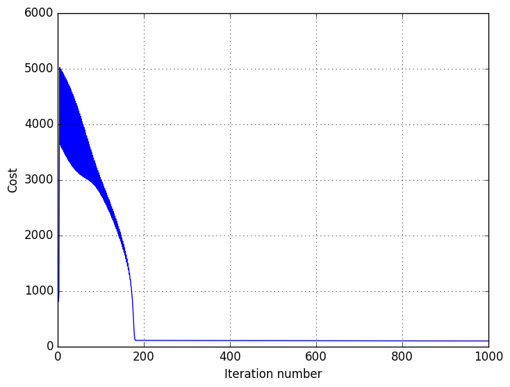
Model is now fitted, let’s see how well our model behaves:

n2 = 100
x_surf = linspace(60,150,n2)
y_surf = linspace(70,160,n2)

# Grid of x and y values
xgrid = repmat(x_surf',n2, 1)
ygrid = repmat(y_surf,  1,n2)

zgrid = zeros(n2,n2)

for ii=1:n2
    for jj=1:n2
        values = vec([1, x_surf[jj], y_surf[ii]])
        zgrid[ii,jj] = sigmoid(O, values)[1]
    end
end

levels = linspace(0, 1, 21)
cp = contourf(xgrid, ygrid, zgrid, levels=levels, linewidth=0.1)
colorbar(cp)

scatter(x_hornet, y_hornet, c="k", marker="+", label="Hornet")
scatter(x_bbee, y_bbee, c="g", marker="x", label="Bumblebee")
axis(:equal)
xlabel("Size of the insect")
ylabel("How terrifying insect looks")
grid()
legend()

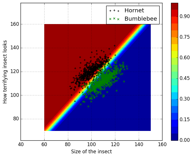
Looks quite nice. If we’d iterated even longer, the region of the most uncertanty would be even slimmer. Do note, that we’re still using linear functions, which results to linear decision surface. One popular example is to use MNIST library, which has images of hand written numbers. You could try to create a model, which recognizes whether the image has a zero or one number. Package can be installed to Julia using package manager.

Conclusion

We’ve seen logistic regression model, which used linear functions, sigmoid function and cost function. Again, one can think a lot of example where this could be valuable (is something dead/alive or with these cards will I win/lose). And how is this connected to neural networks journey in anyway? In my halite model my question was: with the given blocks surrounding my block (which I wanted to move), which is the best direction to move? Moves were presented as numbers: 0 is still, 1 is north, 2 is east, 3 is south and 4 is west, which makes total of 5 choices. I guess you already noted, that logistic regression can only categorize binary values: 0 or 1 (and this is due to the sigmoid function). Magic word here is a Multinomial logistic regression, which enables to categorize multiple values, and it works on the same principle as logistic regression. We’ll explore it later in the series. Up until this point all functions, which we have fitted, have been linear. The decision making in halite was much more of nonlinear nature, which is why in the next post we’ll dive into neural networks. Neural networks transforms our linear functions into nonlinear responses, but we’ll take a look at it next time.