Neural Networks journey: multiclass categorization

May 13, 2017

TL;DR

In this post we’ll cover multiclass categorization problem using support vector machine classifier. All the code in this post is written in Python, version 3.6. I’ve gathered most of the used material from here. It’s very good site, if you want to check out more example and theory.

Multiclass classifier

Before going into neural networks, I thought we should cover multiclass classifier first. In the previous posts we created a binary classifier, which was able to classify two categories (classes): bees and hornets. But what if we want to classify multiple classes, f.ex: lady bugs, bees, butterflies etc. As before, let’s create some data first, so we can visualize the problem.

%matplotlib inline
import numpy as np
import matplotlib.pyplot as plt
import matplotlib
from IPython.display import Image
from IPython.core.display import HTML

matplotlib.rcParams['figure.figsize'] = (15.0, 10.0)

num_of_points =  300

x1 = np.random.normal(-1, 1, num_of_points)
y1 = np.random.normal(-1, 1, num_of_points)
n1 = np.zeros(num_of_points)

x2 = np.random.normal(2, 1, num_of_points)
y2 = np.random.normal(2, 1, num_of_points)
n2 = np.zeros(num_of_points)
n2[:] = 1

x3 = np.random.normal(3, 1, num_of_points)
y3 = np.random.normal(-3, 1, num_of_points)
n3 = np.zeros(num_of_points)
n3[:] = 2

x = []
y = []
n = []
for ni in [x1, x2, x3]:
    x.extend(ni)
for ni in [y1, y2, y3]:
    y.extend(ni)
for ni in [n1, n2, n3]:
    n.extend(ni)

train_input = np.array([x,y]).T
train_output = np.array(n)

perm = np.random.permutation(train_output.shape[0])
train_input_shuffled = train_input[perm]
train_output_shuffled = train_output[perm]

plt.scatter( x1,  y1, marker="+", label="Butterfly")
plt.scatter( x2,  y2, marker="x", label="Beetle")
plt.scatter( x3,  y3, marker="o", label="Grasshopper")
plt.xlabel("Wing span [cm]")
plt.ylabel("Weight [g]")
plt.legend()
plt.grid()

png

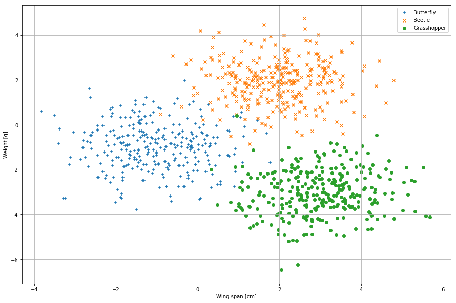
As you can see there are three clusters, each representing one bug. We’ll use the same tools as before, but we only need a proper loss function for this: Support vector machine

Support vector machine

Multiclass classifier

For multiclass classifier there are couple of options, f.ex. support vector machine (SVM) or softmax but we’ll use SVM. SVM is defined as ( ref ):

\begin{equation} L_i = \sum_{j\neq y_i} \max(0, s_j - s_{y_i} + \Delta) \end{equation}

in which $s_i$ is our linear function: \begin{equation} s_j = f(x_i, \theta, b)_j = (\theta x + b)_j \end{equation}

Looks intimidating, how do we use it? $s_j$ represents just the score of the function and $j$ and $y_i$ represent indeces. $y_i$ is special case and represent the correct index (or the correct class). Let’s say we have input vector, which has six (6) elements. We’ll calculate the score using linear function and the output vector has (4) elements, which represent our categories. Let’s say the correct class is index 1 and use it to calculate the loss:

input_vector = np.array([5.2, 1.0, 6.356, 10.1, -4.45, 8.20]).T
theta = np.random.rand(4,6)
beta = np.random.rand(4)
yi = 1
delta = 1

scores = np.dot(theta, input_vector) + beta
print("Score vector: {0}".format(scores))
s_yi = scores[yi]
Li = 0
for j in range(len(scores)):
    if j == yi:
        continue
    score = scores[j] - s_yi + delta
    if score > 0:
        Li += score
print("Score: {0}".format(Li))

Score vector: [ 16.77187651  19.85518302  22.05848935  18.11694353]
Score: 3.203306333209401

Now do note, that in the logistic regression we got only one output value for given set of inputs. Multiclass classifier produces a array, which contains a score for each class. In the example we had a input array which had 6 values and using dot product we got score array which had 4 values or classes. The highest score represents the best guess. When we make a prediction, we select the class which has the highest score using argmax -function.

Loss function represents the fitness of our fit, or the quantity of data loss. But there lies a bug in our code. Suppose we want to minimize the $L_i$ function, which is $0$ . Now the problem arises if $\theta$ is converges to $0$ and that might not be our preferred fit. We’ll need to add a penalty for the $\theta$ too, and in this case, we can use regularization penalty $R(\theta)$ . One of the most common penalties is the L2 norm:

\begin{equation} R = \sum_i \sum_j \theta^2_{i,j} \end{equation}

Now if we add this to loss function, and suppose we have $i$ number of points to fit our model, the total loss function is now:

\begin{equation} L = \frac{1}{N}\sum_i L_i+ \frac{\lambda}{2} R(\theta) \end{equation}

in which $\lambda$ is the regularization strength and $N$ is the number of points. It’s also common to see the $\frac{1}{2}$ in front of the regularization so, so that the derivative will cancels it out. We’ll need the gradient of our loss function for the stochastic gradient algorithm, so here it is:

\begin{equation} \frac{\partial L}{\partial \theta_n} \rightarrow \frac{1}{N}\frac{\partial}{\partial \theta_n}(\sum_i L_i) + \frac{\lambda}{2} \frac{\partial}{\partial \theta_n} (\sum_i \sum_j \theta^2_{i,j}) \end{equation}

Now in order to derivate the $L_i$ we need to use the chain rule:

\begin{equation} \frac{\partial L}{\partial \theta_n} = \frac{1}{N} \frac{\partial L_i}{\partial s_i}\frac{\partial s_i}{\partial \theta_n} + \lambda \theta \end{equation}

Now derivating $L_i$ presents us two cases: one where we derivate $s_j$ and one where we derivate $s_{y_i}$

$\ \frac{\partial L_i}{\partial s_i} = \begin{cases} -(\sum_{j\neq y_i} \mathbb{1}(s_j - s_{y_i} + \Delta))x_i, & \text{i $\equiv y_i$ $\rightarrow$ respect to $s_{y_i}$ }\\ \mathbb{1}(s_j - s_{y_i} + \Delta)x_i, & \text{else } \end{cases} \$

$\mathbb{1}$ is just a function, which just evaluates if the inside is greater then zero function produces value 1 and if not, function produces 0. Now that function is quite long, so let’s make an alias for that:

\begin{equation} \nabla L_i = \frac{\partial L_i}{\partial s_i} \end{equation}

and our final equation is:

\begin{equation} \frac{\partial L}{\partial \theta_i} = \frac{1}{N} \nabla L_i + \lambda \theta \end{equation}

Phew! We’re almost done! Here’s the code:

def svm_loss_function_and_gradient(theta, X, y, delta):
    score_matrix = np.dot(X, theta)
    theta_shapes = theta.shape
    categories = X.shape[1]
    n_points = X.shape[0]
    L = 0.0
    dL = np.zeros(theta_shapes)

    # compute the loss and the gradient
    for i in range(n_points):

        # Select the correct score index
        yi = y[i]

        # Select score row and correct score
        scores = score_matrix[i, :]
        correct_score = scores[yi]

        # Calculate the loss function
        score_row = np.maximum(0, scores - correct_score + delta)
        score_row[yi] = 0
        L += sum(score_row)

        # We want the indeces where score is more than zero
        indeces = np.array(np.nonzero(score_row))[0]

        # Add to gradient
        for idx in indeces:
            dL[:, idx] += X[i, :]
        dL[:, yi] -= len(indeces) * X[i, :]

    # Take the average for L and dL
    L /= n_points
    dL /= n_points
    return L, dL

Fitting the model

In the model I’m not going to use $b$ vector separately, as presented in the equations. Instead I’m going to just add one column to the $\theta$ matrix and an array of ones to the initial X input matrix.

# Theta sizes
D = 3
h = 3

# Theta matrix
theta = 0.01 * np.random.randn(D, h)

# Shuffle the points and add one array
n_points, categories = train_input_shuffled.shape
extra_row = np.ones((n_points, 1))
X = np.hstack([train_input_shuffled, extra_row])
y = train_output_shuffled

# some hyperparameters
step_size = 1e-1
_lambda = 1e-3 # regularization strength

# gradient descent loop
num_examples = X.shape[0]

losses = []
loss_iteration = []
for i in range(500):

    # evaluate class scores, [N x K]
    scores = np.dot(X, theta)

    # Calculate loss and gradient
    L, dL = svm_loss_function_and_gradient(theta, X, y, 1.0)

    # We do not want to add b array, so slice
    dL[:, :-1] += _lambda * theta[:, :-1]

    # Regularization penalty
    reg_penalty = 0.5 * _lambda * np.sum(theta**2)
    total_loss = L + reg_penalty

    # Gradient update
    theta += -step_size * dL

    losses.append(L)
    loss_iteration.append(i)


plt.plot(loss_iteration, losses)
plt.xlabel("Iteration number")
plt.ylabel("Loss")
plt.grid()

png

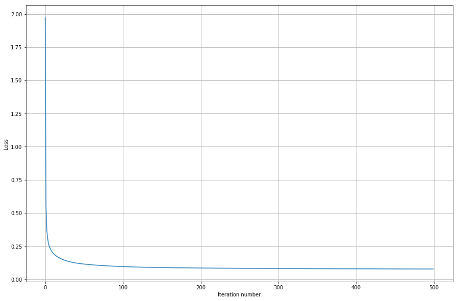
Our function converges to the best value quite fast, and I guess only 200 iterations would have been sufficient. Let’s plot our results!

num_points = 300
x_1 = np.linspace(-3, 6, num_points)
x_2 = np.linspace(-6, 6, num_points)

feed_forward_results = np.zeros((num_points, num_points))
for x_, x_i in enumerate(x_1):
    for y_, x_j in enumerate(x_2):
        k = [x_i, x_j, 1.0]
        scores = np.dot(k, theta)
        value = np.argmax(scores)
        feed_forward_results[y_, x_] = value

X1, Y2 = np.meshgrid(x_1, x_2)
matplotlib.rcParams['figure.figsize'] = (15.0, 10.0)
cs = plt.contourf(X1, Y2, feed_forward_results)
plt.colorbar(cs)
plt.scatter( x1,  y1, marker="+")
plt.scatter( x2,  y2, marker="x")
plt.scatter( x3,  y3, marker="o")
plt.xlabel("Wing span [cm]")
plt.ylabel("Weight [g]")
plt.grid()

png

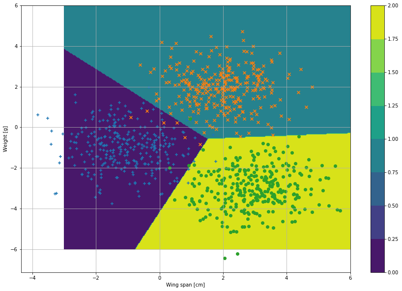
Results look quite good. I wanted to do this post first, since in the next post there’s quite a lot of stuff to go through and trying to fit multiclass things in the post would’ve been quite hopeless. In the next post we’re going to cover at least following subjects: neural network, feed forward, back propagation and softmax classifier. Till next time!