TL;DR;

We’ll start from the basics and first investigate how linear regression is connected with neural networks. In this post all the code is in Julia programming language.

Linear regression

In this post we try to get comfortable with cost functions, computing gradients and learn how to optimize functions over a set of parameters. These are key tools for our upcoming advanced scripts. And yes, there are already tools for calculating this stuff, but if you really want to understand what’s happening under the hood, you have to get your hand dirty or in this case go to the math/code level. Most of the material presented here, can be found from this link.

Let’s first checkup the Wikipedia definition on linear regression:

In statistics, linear regression is an approach for modeling the relationship between a scalar dependent variable y and one or more explanatory variables (or independent variables) denoted X. The case of one explanatory variable is called simple linear regression. For more than one explanatory variable, the process is called multiple linear regression

One could say, that with the given value $x$, how can we predict the value of $y$, f.ex. if I have $x$ number of chickens, how many eggs ($y$) I can get per day (and let’s presume chickens lay eggs linearly). Let’s look at this in an example:

using PyPlot

# This is our magic chicken function
f(x) = 3 + 0.5*x         

# Number of chickens vector
x_prob = collect(1.0:2:20)

# Number of eggs chickens lay
y_prob = f(x_prob)       

# Plotting definitions
grid()
axis(:equal)
scatter(x_prob,y_prob)
title("Chickens vs Eggs per day")
xlabel("Chickens [x]")
ylabel("laid eggs per day [y]")
println("X values: $(x_prob)")
println("Y values: $(y_prob)")

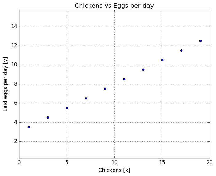
X values: [1.0, 3.0, 5.0, 7.0, 9.0, 11.0, 13.0, 15.0, 17.0, 19.0]
Y values: [3.5, 4.5, 5.5, 6.5, 7.5,  8.5,  9.5, 10.5, 11.5, 12.5]

Now we have a nice line and let’s assume it is a linear and continuous line. As an mental exercise, what would be the $y$ value, if $x$ is 10. Too easy, it’s 8. Ok, but what would be $y$ value, if $x$ is 154.234? Or -2345.455 (minus chickens!). At least my mind can’t calculate that, but that’s ok. We’ll use computer do the heavy lifting.

Linear functions

From the example code above, we used magic function $f(x) = 3 + \frac{1}{2}x$ for calculating $y$ points for us. In linear regression our goal is to find a function $y \approx f(x)$, which would calculate the precise approximation for given values. But what functions to use? We will start with linear functions:

\begin{equation} f(x) = \theta_1 x_1 + \theta_2 x_2 \cdots \theta_n x_n \end{equation}

More compact for for this function presentation would be:

\begin{equation} f(x) = \sum_i \theta_i x_i = \theta^T x \end{equation}

But what are those $\theta$’s? Those are multipliers (just like $3$ and $\frac{1}{2}$ in our magic function) and those are our key to solve this puzzle. Downside is that we will need an algorithm to calculate them ourselves. And how many multipliers do we need? Well, that depends on how many input we have. In our simple example we have number of chickens ($x$) but we’d also want to shift the curve, so we need a constant. That makes two multipliers. Depending what values we choose for our multipliers determines the fit of our curve. We could use trial-and-error way in order find the best multipliers. Just for convenience, I’ll use $x$ and $y$ instead of chickens from now on.

# Hand fitted linear functions
g(x) = 1.1*x        # Function number 1
h(x) = 1 + 0.9*x    # Function number 2
j(x) = 3.5 + 0.5*x  # Function number 2
l(x) = 0.7*x        # Function number 3

# x values
x = collect(1:2:20)

# y values
y_g = g(x)
y_h = h(x)
y_j = j(x)
y_l = l(x)

# Plot definitions
grid()
axis(:equal)
scatter(x_prob, y_prob)
plot(x, y_g)
plot(x, y_h)
plot(x, y_j)
plot(x, y_l)
title("Curves fitted by hand")
xlabel("X")
ylabel("Y")

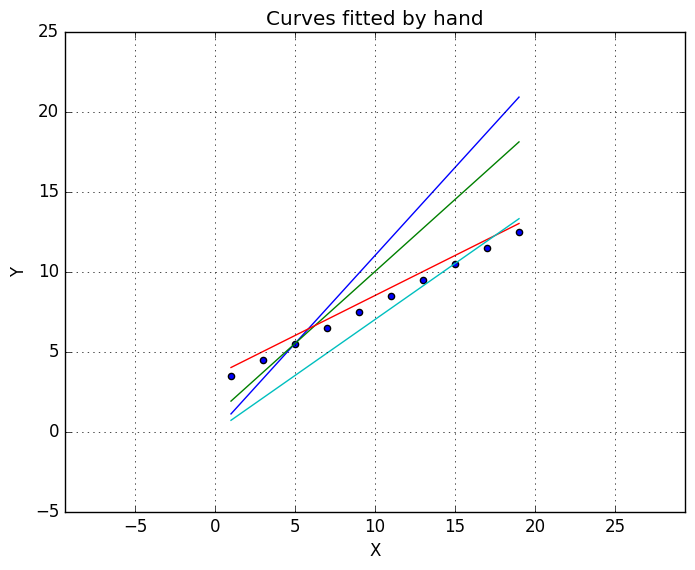
Well, it’s something. But we should have something to determine, how good is our fit! From the plot above, I’d say the red line is the best of line. I don’t have any numbers or data to back up my conclusion, so it’s only a hunch. More important question is: is it the best fit we can achieve? And looking at the graph is quite obvious we could get better fit. Next we’ll take a look at cost function.

Cost function

When you face a question: how good is this or how well is this performing, you need a cost function (also called as loss function). Number of mathematicians have defined various cost functions for different problems (see here for more examples) but we’ll use least squares loss function:

\begin{equation} J(\theta) = \frac{1}{2}\sum_i(f(x^{(i)})-y^{(i)})^2 \end{equation}

I’ll just apply function $f$ directly inside $J$, we’ll be using this formula later.

\begin{equation} J(\theta) = \frac{1}{2}\sum_i(\theta^T x^{(i)} - y^{(i)})^2 \end{equation}

This function basically tells us: if I apply $x$ to function f, how much is it off from true value $y$. If $f(x) \equiv y$, function $J$ returns a zero. If $f(x) \neq y$, function $J$ produces something positive, due to the power of 2. We can conclude, that the best fit can be acquired, when our cost function produces zero. Let’s plot this so we can study it more closely.

# Cost function
function cost(O, x, y)
    return 1/ 2. * sum((O' * x - y).^2)
end

# Let's fix x and y
x = 2.0
y = 5.0

# Range of theta values
O = linspace(-2, 6, 100)

# Cost for each theta value
cost_values = [cost(o, x, y) for o in O]

# plot definitions
grid()
title("Cost function plot, when x=2 and y=5")
xlabel("theta values")
ylabel("Cost function values")
plot(O, cost_values)

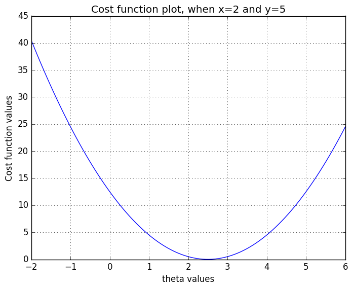
In the plot above is demonstrated how cost function behaves with various $\theta$ values. It can be seen that the best fit is achieved, when $\theta = 2.5$. In the plot I’ve only added one point pair $(x, y) = (2, 5)$. But this is example is too easy! What about the sum function and vector notations inside cost function? If you have multiple points, which you would like to fit, you’ll calculate cost for each $(x,y)$ pair and sum all the costs, which will give you the total fit of your function. If all the points reside on a straight line, your best fit has a total cost of 0 and if your points have little variance, your total cost is something above 0. Final piece in our puzzle is to create a function, which will find the minimum value for our cost function. If you’ve been at a math class, you’ve might hear that minimum value for the function can be found, where the derivative is zero (and now that we have quite easy cost function, which happens to be a convex function, the minimum value is the global minimum). For this task, there are again couple of choices (list of python minimizer can be found f.ex. here) but we’ll are so hard core, we’ll implement gradient descent algorithm ourselves (it’s one of the most simplest algorithms for optimization problems and we’ll use it also in the neural network post).

Gradient descent

Last part is to create a minimization algorithm for our cost function. We’ll use gradient descent for this job, which is defined as:

\begin{equation} x_{n+1} = x_n - \gamma \nabla f(x_n) \end{equation}

in which $\gamma$ is a step size and $\nabla f(x_n)$ is the direction. With $\gamma$ we can decide, how large steps we’re taking each iterations, but this should be quite small. If $\nabla$ operation is not familiar to you, you can find definition f.ex. here, but the short answer is that it calculates derivatives for all function variables. And when derivative is calculated, it tells us in which direction is the steepest descent of the function. Let’s look at the gradient with an example, how it actually behaves:

using ForwardDiff

# Our target function for contour plot
g(x) = (2 - x[1])^2 + (3 - x[2])^2

# Gradient of function g
∇g(x) = ForwardDiff.gradient(g, x)

# x and y ranges
n = 100
x = linspace(-3,7,n)
y = linspace(-3,5,n)

# Grid of x and y values
xgrid = repmat(x',n,1)
ygrid = repmat(y,1,n)

# initialization for z values
z = zeros(n,n)

for ii=1:n
    for jj=1:n
        z[ii,jj] = g([x[jj], y[ii]])
    end
end

fig = figure("pyplot_subplot_mixed",figsize=(10,3)) # Create a new blank figure

# Creating 1x2 subplot
subplot(121)

# Calculating 3 gradients
x_points = [0, 0, 3]
y_points = [3, 0, 3]
dx = []
for (xi, yj) in zip(x_points, y_points)
    p21, p22 = (xi,yj)
    g1 = ∇g([p21; p22])
    annotate("",
        xy=[p21, p22],# Arrow tip
        xytext=[p21 + g1[1], p22 + g1[2]], # Text offset from tip
    arrowprops=Dict("facecolor"=>"black"))
    push!(dx, g1[1])
end

# Plotting contour
cp = contourf(xgrid, ygrid, z, linewidth=2.0)

# Plot definitions
title("Contour + gradients as arrows")
colorbar(cp)
ylim([-3, 5])
xlim([-3, 6])
xlabel("x")
ylabel("y")
axis(:equal)
grid()

# Plotting red dashed line
plot(x, [3 for xx in x], "r--")
subplot(122)

# Red dashed line in right side plot
y_1D = 3.0
z_1D = [g([xx, y_1D]) for xx in x]
plot(x, z_1D, "r--")

lin_func(x, a, b) = a + b*x
plot(x, [lin_func(xx, 4, dx[1]) for xx in x])
plot(x, [lin_func(xx, -5, dx[3]) for xx in x])

title("1D cut from contour")
grid()
ylim([-3, 5])
xlim([-2, 6])
xlabel("x")
ylabel("z")

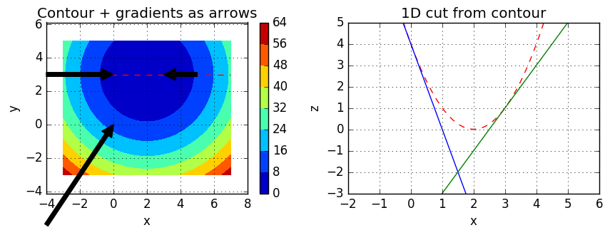
Plots might look a bit confusing, but let’s take a look. In our example, contour is plotted using function:

\begin{equation} g(x) = (2 - x_1)^2 + (3 - x_2)^2 \end{equation}

I don’t always like to do everything by hand, so I cheated a bit and calculated gradient with ForwardDiff package. However, if you want to use analytical gradient, you can use this:

\begin{equation} \nabla g(x) = \left[ \begin{array}{c} -2(2 - x_1) \\ -2(3 - x_2) \end{array} \right] \end{equation}

In the left plot is the contour of our function $g$. Colors represent the function values, which we shall call as $z$. As you can see, blue color represent values below 8 in our contour, red color values over 56 and other colors values withing [8, 56]. Black arrows are gradients at given $(x, y)$ points: (0, 3), (3, 3) and (0, 0). You can see, that the size of the arrow depends on the strength of the gradient. I also wanted to make a 1D plot from contour for demonstration purposes. In the right side plot the red dash line represents the values in the contour plot. The blue line is the gradient at point (0, 3) and the green line is the gradient at (3, 3). It can be seen that steepness the line and the size of the arrow correlate with these two plots. However, from the left plot is more obvious, which direction the gradient points to. An it can be seen all the gradients point to the location, where lies the minimum value. So, in our gradient descent, gradient determines the direction and the $\gamma$ determines the step size. Gradient has to be calculated for each iteration, but $\gamma$ has to be chosen. We’ll use 0.001 and hope it will converge within a decent amount of time.

Now that I’ve got you all confused and dazed, we can return to our regression. For our gradient decent, we need to calculate the gradient of the cost function. I’ll be using ForwardDiff in my code, but here’s the analytical gradient, if you’re curious:

\begin{equation} \frac{\partial J(\theta)}{\partial \theta_j} = \sum_i x_j^{(i)} (\theta^T x^{(i)}-y^{(i)})^2 \end{equation}

Model

Ok, finally we can assembly our model. Let’s summarize, what we’re using:

Linear functions:

\begin{equation} f(x) = \theta^T x \end{equation}

Cost function and it’s gradient:

\begin{equation} J(\theta) = \frac{1}{2}\sum_i(\theta^T x^{(i)} - y^{(i)})^2, \hspace{1cm} \frac{\partial J(\theta)}{\partial \theta_j} = \sum_i x_j^{(i)} (\theta^T x^{(i)}-y^{(i)})^2 \end{equation}

Gradient descent for searhing the minimum value: \begin{equation} x_{n+1} = x_n - \gamma \nabla f(x_n) \end{equation}

Let’s start cracking!

using ForwardDiff
using PyPlot

# Cost function
# Note! O, x and y are row vectors, with size (n)
function cost(f, y)
    return 1/ 2. * sum((f .- y).^2)
end

# naive Gradient Descent algorithm
function grad_desc(x, γ, grad_f; max_iter=10000)
    for i=1:max_iter
        x = x - γ * grad_f(x)
        if all(abs(grad_f(x)) .< 1e-5)
            return x
        end
    end
    println("Could not converge to global minimum within $(max_iter) iterations!")
    return x
end

# Our linear function f(x, a, b) = a + b*x
#
# Just for fun, you could also make it: f(x, O) = O' * x
# but in this formulation, you'll need to add integer 1 to x, which takes into
# account the variable a. Also, make sure your vectors are the right shape (row vs column vectors)
f_fit(O, x) = [O[1]+O[2]*x_ for x_ in x]

# x_prob and y_prob can be found from the beginning of the post (chicken vectors)
# Also, forcing x_prob and y_prob to 1D-vectors
x_vec = vec(x_prob)
y_vec = vec(y_prob)

# Let's make an alias, just so our function names match
J(O) = cost(f_fit(O, x_vec), y_vec)

# Gradient
∇J(x) = ForwardDiff.gradient(J, vec(x))

# We have no idea of optimum multiplier, so let's just initialize random vector
O = rand(2)
γ = 0.001

# Calculating optimal O values
O_optim = grad_desc(O, γ, ∇J)

print("Optimal values: $(O_optim)")
title("x and y scatter plot with fitted curve")
xlabel("x")
ylabel("y")
grid()
scatter(x_vec, y_vec)
plot(x_vec, f_fit(O_optim, x_vec))

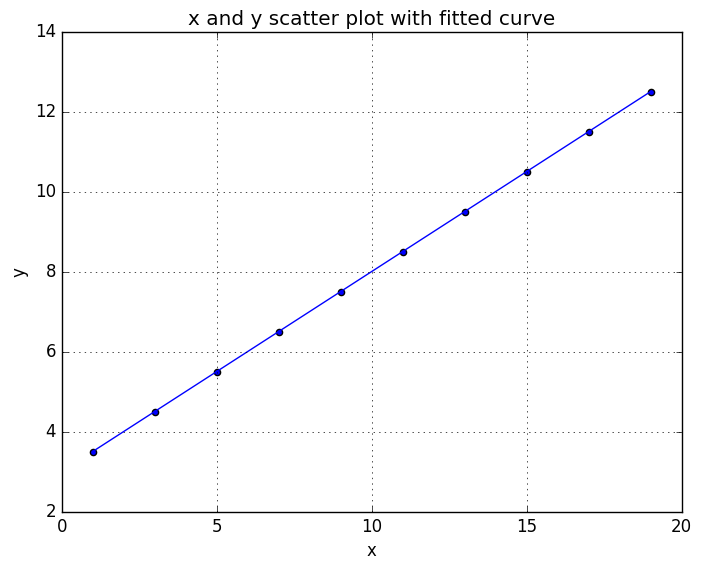
Optimal values: [2.9999959525127005,0.5000003048879387]

And fits like a glove! From the printed optimal values, you can check that the constant is almost 3 and slope 0.5, which are the same as what we defined earlier in the post. Now that we have our example working, we can try out something a bit harder. In the following example I used BFGS optimizer (definitions for BFGS), because our gradient descent implementation wasn’t converging fast enough. Main difference between BFGS and gradient descent is that BFGS requires the calculation of Jacobian. In this example it’s ok (also converges faster), but for neural network problems turns out to be quite unefficient solver. But let’s not dig in to that and just go to the code:

using PyPlot
using Optim
using Distributions

x_dist = rand(Normal(100, 7), 600);

# Magic function for generating data
f(x) = 50 + 0.7 *  x .+ rand(Normal(1, 7), length(x_dist)) .* rand(length(x_dist))

# Value for training data
y_dist = f(x_dist);

# Cost function and gradient
J(O) = cost(f_fit(O, x_dist), y_dist)

# Calculate optimum value
results = Optim.optimize(
    J,
    zeros(2),
    BFGS(),
        OptimizationOptions(
            autodiff   = true
        )
    )

O_optim = Optim.minimizer(results)

fig = figure()

# Plotting x and y distributions
scatter(x_dist, y_dist)

# Plotting our fitted curve
x_linspace = linspace(60, 140, 100)
fit_y = f_fit(O_optim, x_linspace)
plot(x_linspace, fit_y, "r--")

# Some plot definitions
axis(:equal)
grid()
title("Height and weight of mystic space bears")
xlabel("Height [cm]")
ylabel("Weight [Kg]")
println("Optimal values: $(O_optim)")
println("Value for cost function: $(J(O_optim))")

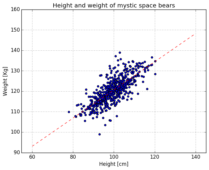
Optimal values: [51.75353640575521,0.6886400445282604]
Value for cost function: 4996.621665905874

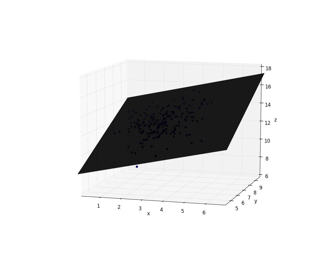
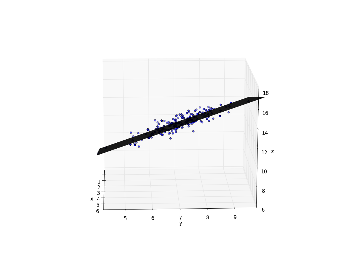
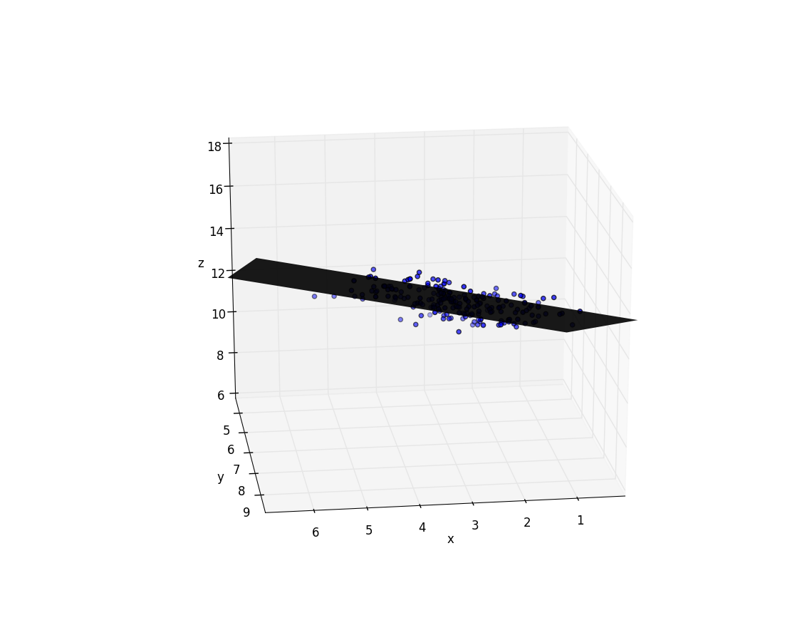
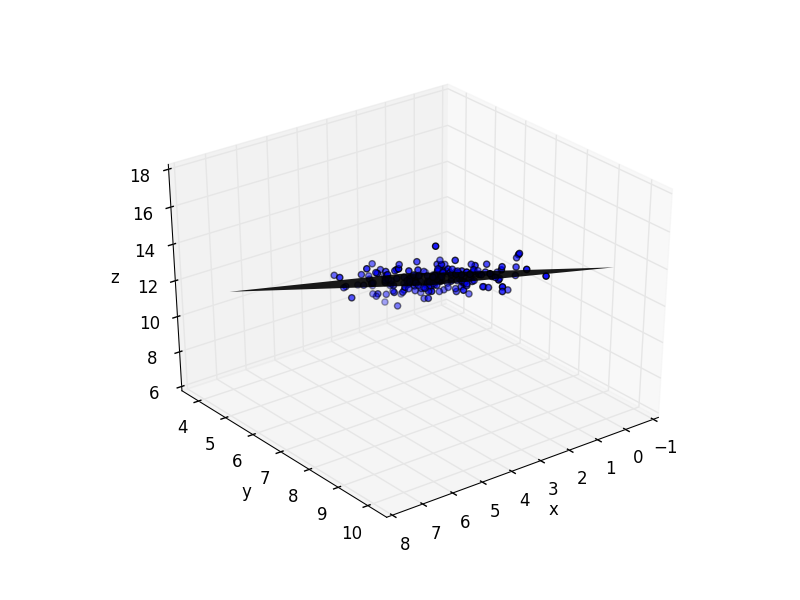
Now the multipliers aren’t the same as in the magic function and the cost function is far from zero, due to the variance in data. But this is the best fit we can achieve with our linear model. We’ve only been fitting one input variable $x$, so I’ll add just one more example, if you’d have two inputs ($x_1, x_2$).

using PyPlot
using Optim
using Distributions

# Cost function again
function cost(f, y)
    return 1/ 2. * sum((f .- y).^2)
end

# Our linear function. Now we'll add ones to x matrix to take into account
# the constant
f_fit(O, x) = vec(O' * x)

# Number of samples
num_of_points = 200

# Magic function for generating data
f(x) =  5 + 1.0 * x[2] + 0.5 * x[3] + rand(Normal(-1, 0.5))

# Values for training data
xs = zeros(3, num_of_points)
xs[1, :] = 1.0                              # Constant
xs[2, :] = rand(Normal(7,1), num_of_points) # multiplier for x_1
xs[3, :] = rand(Normal(3,1), num_of_points) # multiplier for x_2

# Empty vector for y-values
ys = zeros(num_of_points)

# Calculate y-values
for ii=1:num_of_points
    ys[ii] = f(xs[:, ii])
end

# Cost function initialization
J(O) = cost(f_fit(O, xs), ys)

# Calculation using BFGS
results = Optim.optimize(
    J,
    zeros(3),
    BFGS(),
        OptimizationOptions(
            autodiff   = true
        )
    )

O_optim = Optim.minimizer(results)
println("Optimum multipliers $(O_optim)")

fig = figure()


# Creating some plotting data
# x & y grid
n = 10
x = linspace(0, 7, n)
y = linspace(4, 10, n)
xgrid = repmat(x',n,1)
ygrid = repmat(y,1,n)
z = zeros(n,n)

# z-values
for i in 1:n
    for j in 1:n
        z[i, j] = f_fit(O_optim, [1, y[i], x[j]])[1]
    end
end

# Plotting surface
surf(xgrid,ygrid,z, linewidth=0, shade=false, cmap=ColorMap("gray"), alpha=0.9)

# Plotting points
ax = scatter3D(xs[3, :], xs[2, :], ys)

xlim([0, 7])
ylim([4, 10])
axis(:equal)

Optimum multipliers [4.152901600257437,0.9680090333702178,0.5540136524257544]

Conclusion

In this post we’ve seen a linear regression model, which used linear functions, cost function and couple of optimizers. There are bunch of use cases for linear regression from statistics to stock markets (For more examples, I’d use duckduckgo or Google). And how is this connected to neural networks in anyway? In neural networks we’re also interested in solving the optimal multipliers for the model, so the basic question remains the same: How can I fit this neural model to my data. In the follow up post we’ll take a look into logistic regression. It has same principles as linear regression, but it can be used to solves a bit different kind of problems.