Calculating element surface area
Background
A while ago I had a problem of calculating element surface areas from finite element model. Let’s illustrate the problem:
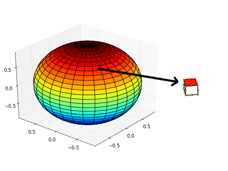
As you can see there’s a ball, which is constructed from a finite number of elements (let’s make an assumption, that these elements are brick elements, just like the one that the arrow is pointing at). Each element is constructed from 20 nodes (the yellow points). The objective is to calculate surface area of the red face from the element. The information we have are the coordinates of the nodes and the element type. My first approach was to google for a solutions. I found algorithms for calculating surface areas in a plane using curves, analytical equations for triangles & boxes etc. Only problem with these algorithms were that they defined in 2D but the problem we have here is to calculate surface area in 3D space. Since I didn’t find any easy solutions (I don’t say there isn’t one, I just didn’t have the patience to search deeper), so here’s an solution I tinkered using Julia programming language.
Theory
Since the problem was related to finite element method, I think we’ll make a short introduction to method:
The finite element method (FEM) is a numerical technique for finding approximate solutions to boundary value problems for partial differential equations. It is also referred to as finite element analysis (FEA). FEM subdivides a large problem into smaller, simpler, parts, called finite elements. The simple equations that model these finite elements are then assembled into a larger system of equations that models the entire problem. FEM then uses variational methods from the calculus of variations to approximate a solution by minimizing an associated error function. (ref Wikipedia)
In finite element method field variables are integrated over volume or area, depending on the simulation dimensions. But calculating variables (e.g. stiffness tensor) can prove to be difficult to calculate, since:
-
The construction of shape functions that satisfy consistency requirements for higher order elements with curved boundaries becomes increasingly complicated
-
Integrals that appear in the expressions of the element stiffness matrix and consistent nodal force vector can no longer be evaluated in simple closed form.
Luckily these obsticles were overcome through the concepts of isoparametric mapping and numerical quadrature. Combining these ideas transformed the field of finite element methods during the 1960’s. Let’s dig in. (ref. University of Colorado)
Isoparametric mapping
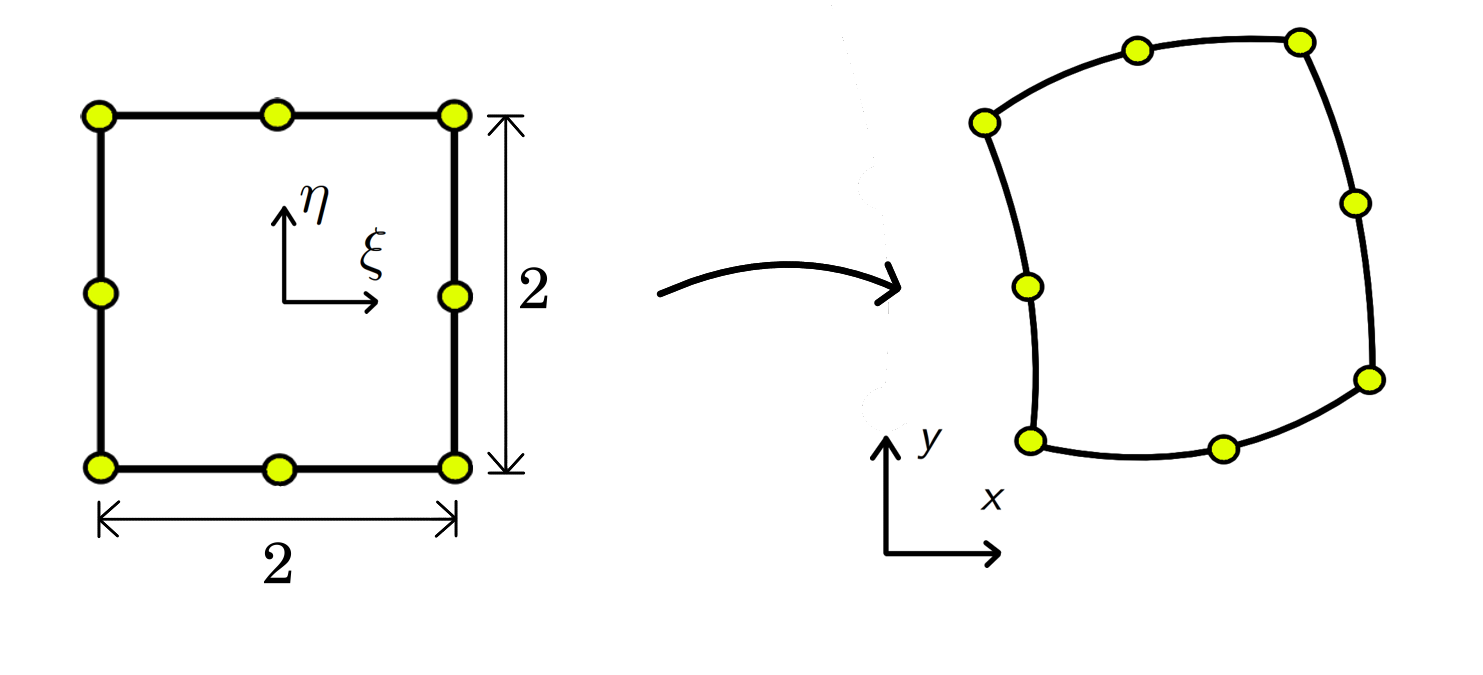
As you can see in the picture, the goal is to map element from local coordiantes system to global coordinate system. This can be achived with the use of shape functions.
Shape functions
Shape functions or basis fuctions are used to obtain an approach solution to the exact solution (ref. Kratos). Shape functions can represent both the element geometry and the problem unknowns, hence the name isoparametric element (“iso” means equal). In the Finite Element Method a lineal combination is used to interpolate the solution:
\begin{equation} x = \sum_{i=1} N_i x_i \end{equation}
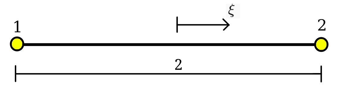
in which are the shape functions (functions of and ) and are coordinates of a node. The number of shape functions used for given element corresponds to the number of nodes in an element. For example, linear 1D bar element can be defined as:
Let’s plot this shape function within element’s area
using PyPlot
subplot(2,1,2)
N_lin_bar(ξ) = [(1-ξ)/2., (1+ξ)/2.]
x_axis = linspace(-1, 1, 10)
n_vals = map(x-> N_lin_bar(x), x_axis)
N1 = map(x-> x[1], n_vals)
N2 = map(x-> x[2], n_vals)

plot(x_axis, N1, label="N1")
plot(x_axis, N2, label="N2")
legend()
grid()
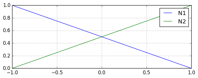
As you can see , which is the first element in , corresponds to the node #1, since it gains the value of 1 in that node. , which is the second element in , corresponds to the node #2. Now that the shape functions work, let’s try to interpolate x coordinate within the element.
# example coordinates
x_example = [3, 5]
println("Coordinate in first node:            $(dot(N_lin_bar(-1), x_example))")
println("Coordinate in the middle of element: $(dot(N_lin_bar(0), x_example))")
println("Coordinate in second node:           $(dot(N_lin_bar(1), x_example))")
Coordinate in first node:            3.0
Coordinate in the middle of element: 4.0
Coordinate in second node:           5.0
Ok, cool thing. There are many documentations/sites, where to acquire shape functions for different shapes but I’ll be using functions from code aster documentation. Now let’s try the same with a square with four (4) nodes:
# example coordinates
x_coords = [0, 2, 2.3, 0]
y_coords = [0, 0.5, 2, 2]

# shape functions
N_quad_4(η, ξ) = [  0.25 * (1 - ξ) * (1 - η),
                    0.25 * (1 - ξ) * (1 + η),
                    0.25 * (1 + ξ) * (1 + η),
                    0.25 * (1 + ξ) * (1 - η) ]

# calculate shape functions values in various locations in local coordinates
f_n_1 = N_quad_4(-1, -1)
f_n_2 = N_quad_4(0 ,0)
f_n_3 = N_quad_4(1, -1)
f_n_4 = N_quad_4(1, 1)

# Plotting twice just to get a closed loop
plot(x_coords, y_coords)
plot([x_coords[end], x_coords[1]], [y_coords[end], y_coords[1]], "b")
scatter(x_coords, y_coords);

println("Coordinates in first node:            x = $(dot(f_n_1, x_coords)),   y = $(dot(f_n_1, y_coords))")
println("Coordinates in the middle of element: x = $(dot(f_n_2, x_coords)), y = $( dot(f_n_2, y_coords))")
println("Coordinates in second node:           x = $(dot(f_n_3, x_coords)),   y = $(dot(f_n_3, y_coords))")
println("Coordinates in third node:            x = $(dot(f_n_4, x_coords)),   y = $(dot(f_n_4, y_coords))")
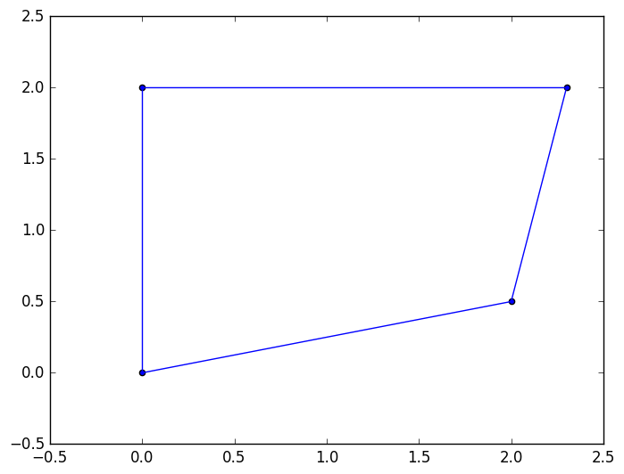
Coordinates in first node:            x = 0.0,   y = 0.0
Coordinates in the middle of element: x = 1.075, y = 1.125
Coordinates in second node:           x = 2.0,   y = 0.5
Coordinates in third node:            x = 2.3,   y = 2.0
Gaussian quadrature
Now that we can get the coordinates within element, we can focus on integrating the area. Let’s say we want to integrate some field variable over surface:
\begin{equation} F = \int_{\Omega_A} f(x,y)\hspace{2mm} dA \end{equation}
Using shape functions and integration rules we can transform area integration:
\begin{equation} \int_{\Omega_A} f(x,y)\hspace{2mm} dA = \int_{-1}^1\int_{-1}^1 f(\eta, \xi) \det J\hspace{2mm}d\eta d\xi \end{equation}
in which is jacobian (as seen here in eq. 17.8). Now equation can be finalize using gaussian quadrature:
\begin{equation} \int_{-1}^1\int_{-1}^1 f(\eta, \xi) \det J\hspace{2mm}d\eta d\xi= \sum_{n=1}^{n_p} f(\eta_p, \xi_p) \det J(\eta_p, \xi_p) W_p \end{equation}
Now that we’re only integrating the surface area, we’ll be using only:
\begin{equation} Area = \sum_{n=1}^{n_p} \det J(\eta_p, \xi_p) W_p \end{equation}
For more info on formulation, check out here and wikipedia. But without further due, let’s try our area calculation formula.
using ForwardDiff

# Shape functions for a square with four nodes.
# Check more information on code aster documentation
N_quad_4(η, ξ) = [  0.25 * (1 - ξ) * (1 - η),
                    0.25 * (1 - ξ) * (1 + η),
                    0.25 * (1 + ξ) * (1 + η),
                    0.25 * (1 + ξ) * (1 - η) ]

# Wrapping function
N_wrap_quad(x) = N_quad_4(x[1], x[2])

# I'm a bit lazy and I'll use ForwardDiff to calculate jacobian function
dN_quad = ForwardDiff.jacobian(N_wrap_quad);
# Function for calculating surface area in 2D
function calculate_surface_2D(x, y, dN, points, weigths)
    area = 0.0
    for i=1:length(points)      # integration points in η-direction
        for j=1:length(points)  # integration points in ξ-direction

            # Selecting integration points and weights
            i_point = points[i]
            j_point = points[j]
            i_weight = weights[i]
            j_weight = weights[j]

            # Calculating derivatives
            DN = dN([i_point, j_point])

            # Picking vectors
            dNdη = DN[:, 1]
            dNdξ = DN[:, 2]

            # Jacobian
            J = [dot(x, dNdη) dot(x, dNdξ);
                 dot(y, dNdη) dot(y, dNdξ)]

            # Area calculation
            area += i_weight * j_weight * det(J)
        end
    end
    area
end

# Example coordinates
x = Float64[0, 1, 1, 0]
y = Float64[0, 0, 1, 1]

# Integration points and weights for gaussian quadrature
points = [-sqrt(1/3.), sqrt(1/3)]
weights = [1, 1]

calculated_area = calculate_surface_2D(x, y, dN_quad, points, weights)
println("Area of 1x1 square: $calculated_area")
Area of 1x1 square: 1.0
3D formulation
Cool story bro, but how about in 3D? We’ll, in 3D space the calculation is almost the same, except with a small twist. Calculating the surface area of a square is done using formula:
\begin{equation} Area = height \cdot width \end{equation}
Using vectors to perform this task can prove to be a bit more convinient. Calculating surface area with vectors is done using cross product (ref. Math insight).
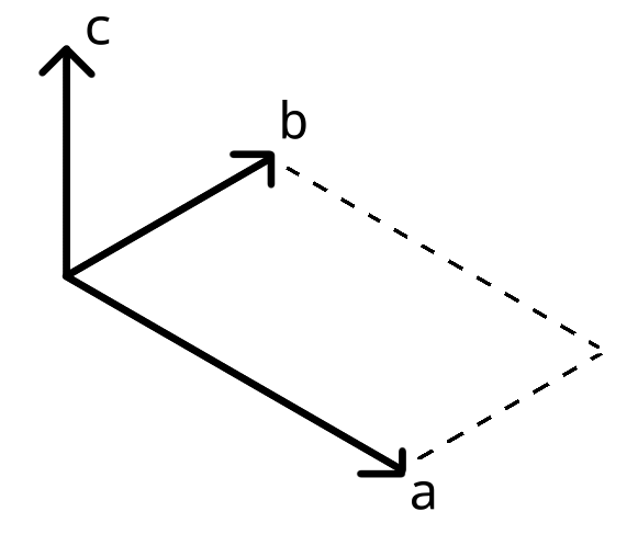 \begin{equation}
c = a \times b = \begin{vmatrix}
i & j & k \\
a_i & a_j & a_k \\
b_i & b_j & b_k
\end{vmatrix}
\end{equation}
\begin{equation}
Area = \begin{vmatrix} c \end{vmatrix}
\end{equation}
\begin{equation}
c = a \times b = \begin{vmatrix}
i & j & k \\
a_i & a_j & a_k \\
b_i & b_j & b_k
\end{vmatrix}
\end{equation}
\begin{equation}
Area = \begin{vmatrix} c \end{vmatrix}
\end{equation}
Taking the norm of vector reveals the surface area defined by vectors & . Now, let’s make an assumption, that components are 0. Using the determinant rules, equation can be simplified into:
\begin{equation} c = \begin{vmatrix} a_i & a_j \\ b_i & b_j \end{vmatrix} k \end{equation}
Using the determinant notation, this can be formulated as:
\begin{equation} Area = \begin{vmatrix} \det \begin{pmatrix} \begin{bmatrix} a_i & a_j \\ b_i & b_j \end{bmatrix} \end{pmatrix} \end{vmatrix} \end{equation}
Previously in 2D formulation we can see how the determinant of the jacobian was used to calculate the surface area. In the 3D formulation we’ll use all and components. Coordinates are projected on xy-, yz- and xz-planes and individual surface areas calculated on these planes. The total surface area is calculated as a norm of these smaller surface areas
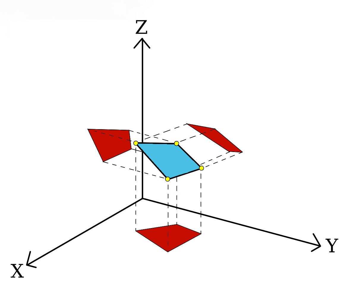
More material for enthusiastic reader can he found from here
"""
Function for rotating coordinates around axis

Reference: http://www.codeproject.com/KB/GDI-plus/eulerangle.aspx?msg=2635186
"""
function rotate_cube(x,y,z,angle)
    x_ = []
    y_ = []
    z_ = []
    rot_x(ϕ) = [1      0      0
                0  cos(ϕ) sin(ϕ)
                0 -sin(ϕ) cos(ϕ)]

    rot_y(ϕ) = [ cos(ϕ) 0 sin(ϕ)
                     0  1      0
                -sin(ϕ) 0 cos(ϕ)]

    rot_z(ϕ) = [ cos(ϕ) sin(ϕ) 0
                -sin(ϕ) cos(ϕ) 0
                     0       0 1]
    rotation_matrix = rot_x(angle) * rot_y(angle) * rot_z(angle)
    for i=1:length(x)
        crd = rotation_matrix * [x[i], y[i], z[i]]
        push!(x_, crd[1])
        push!(y_, crd[2])
        push!(z_, crd[3])
    end
    x_, y_, z_
end

"""
Surface calculation function
"""
function calculate_surface_3D(x, y, z, dN, points, weigths)
    area = 0.0
    for i=1:length(points)      # Integrating η direction
        for j=1:length(points)  # Integrating ξ direction

            # Selecting values
            ip = points[i]
            jp = points[j]

            iw = weights[i]
            jw = weights[j]

            # Calculating derivatives
            DN = dN([ip, jp])

            # picking derivatives
            dNdη = DN[:, 1]
            dNdξ = DN[:, 2]

            # Coordinates
            dx = [dot(x, dNdη), dot(x, dNdξ), 0]
            dy = [dot(y, dNdη), dot(y, dNdξ), 0]
            dz = [dot(z, dNdη), dot(z, dNdξ), 0]

            # Calculate lengths of the normals
            dAdx = norm(cross(dy, dz))
            dAdy = norm(cross(dz, dx))
            dAdz = norm(cross(dx, dy))

            # Area calculation
            area += iw * jw * norm([dAdx, dAdy, dAdz])
        end
    end
    area
end

# Coordiantes: 1x1 plate
x = Float64[0, 1, 1, 0]
y = Float64[0, 0, 1, 1]
z = Float64[0, 0, 0, 0]

# Just to make sure, that function calculates the right answer,
# let's rotate the plate 45 deg around all axis
x_, y_, z_ = rotate_cube(x, y, z, 45.*pi/180.)

# Integration points and weights for gaussian quadrature
points = [-sqrt(3/5.), 0.0, sqrt(3/5.)]
weights = [5/9., 8/9., 5/9.]

face_area = calculate_surface_3D(x_, y_, z_, dN_quad, points, weights)
println("Area of the selected face: $face_area")
Area of the selected face: 1.0
And that’s about it, hopefully I didn’t leave any bugs or mistakes. Picking different shape functions enables calculating various shapes. Now, in my original problem I had 20 nodes in one hexagon, which meant that I just had to pick the right nodes in right order, pick shape functions for Quad8 and use following algorithm to calculate the surface area.
Note
Since we’re using shape functions to calculate the surface area, there’s a catch: Shape functions interpolate the coordinates inside element area, and if element happens to be distorted (not exactly the same shape as what shape functions define) there’s a bit error in the solution: more distortion, more the error.